Large Language Models

The following video course has such stunning graphics that we will use it to illustrate everything here.
Images are screenshots from the following videos.
Deep Learning video course by Grant Sanderson.
- Intro: Large Language Models explained.
- Chapter 5: Transformers, the tech behind LLMs.
- Chapter 6: Attention in transformers.
- Chapter 7: How might LLMs store facts
- Missing: Training.
Large language model (LLM)
Attention mechanism
Transformer model (started the AI explosion in 2017)
"Attention Is All You Need" paper (2017).
Generative pre-trained transformer (GPT)
Reinforcement learning from human feedback (RLHF)

Intro: Large Language Models explained

Intro: Large Language Models explained.

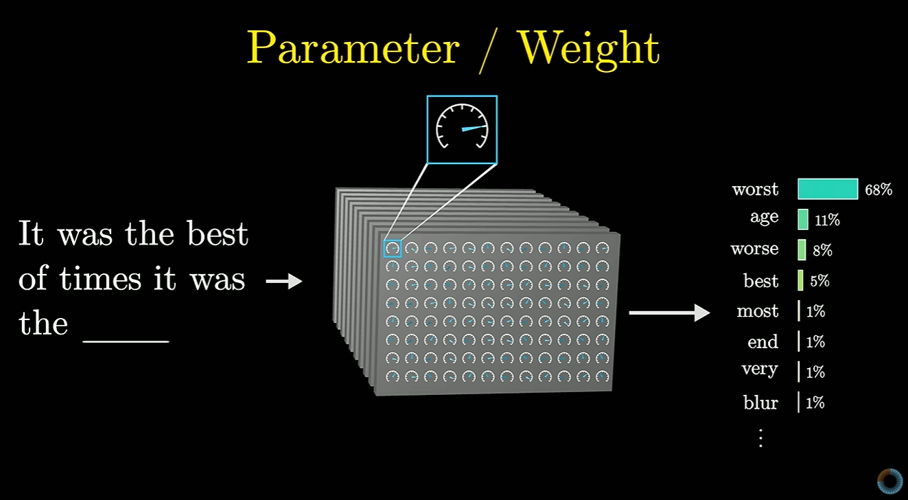
Pre-training for Generating text. Learning probabilities of next word as weights.

Training set can be random human texts. Vast numbers of them.
Can pass in sentence minus one word. Or page of text minus one word.
Compare machine prediction with correct answer - true last word - and adjust weights.
Texts provide contradictory examples of next word. No single answer. So learn probabilities.
One issue is whether LLM when generating text should always pick the no.1 probability only. Why might that be a bad idea?

Chapter 5: Transformers, the tech behind LLMs

Chapter 5: Transformers, the tech behind LLMs.

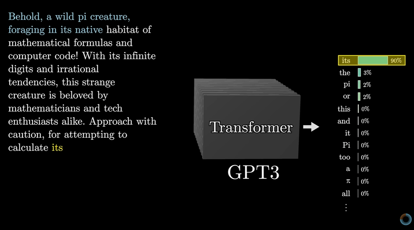
"Predicting" an entire story from seed text. Predict one word. Feed back in. Predict another word. Feed back in.
I like the way he says it feels like this should not really work, but it can.

Break input into pieces - tokens.
Easy to visualise tokens as words, and the graphics will do so. But a token could be part of a word.
Each token is mapped to a (very large) vector of numbers.
This vector encodes the token's "meaning".
Token vector length ("hidden dimension") can be very large. e.g. In largest version of GPT-3, vector length was 12,288 numbers.
To help the architecture, these vectors are all the same length.
Words with similar meanings have similar vectors, like similar locations in n-dimensional space.

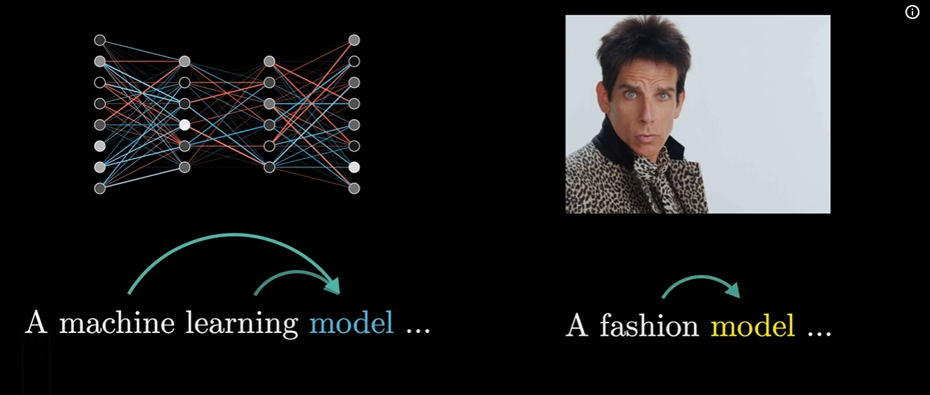
Attention mechanism is used for nearby tokens to update the numbers (i.e. the meaning) of the vector of a token.
Here the vector for "model" ends up entirely different in the two situations.

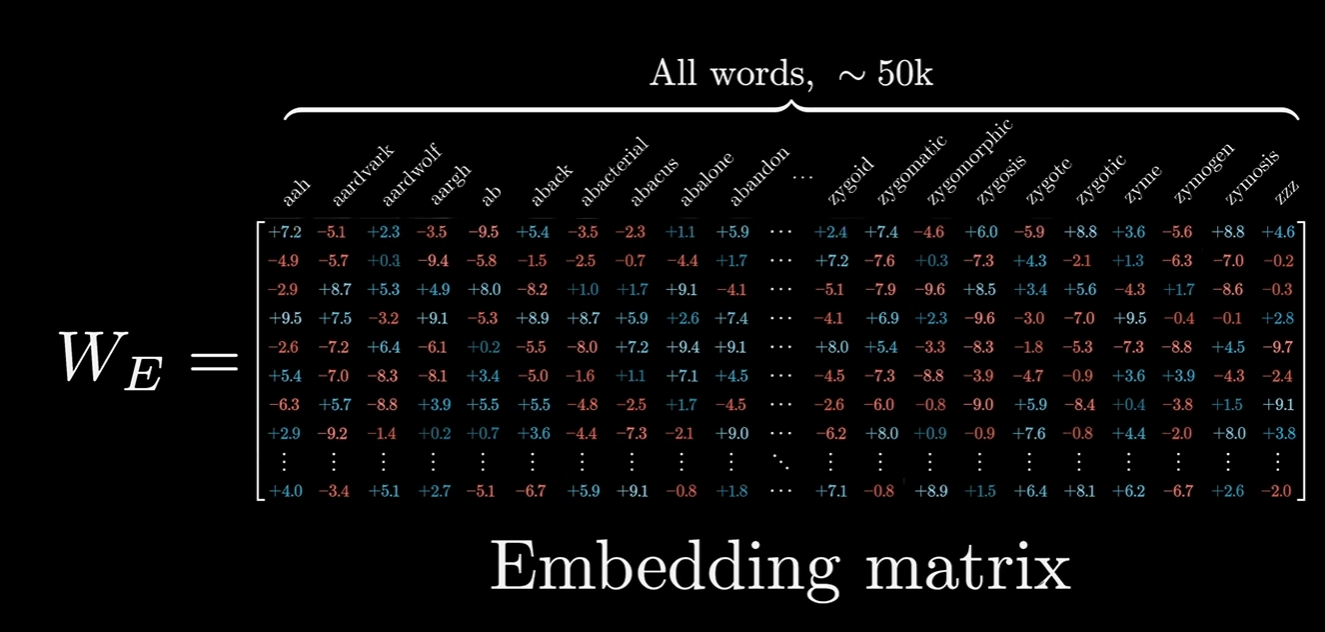
An embedding matrix is a trainable lookup table that converts tokens into high-dimensional numeric vectors.

See long history of Word embedding in NLP.
As the model learns, it embeds words as points in n-dimensional space (maybe thousands of dimensions). The way this happens is that different dimensions take on different meanings.

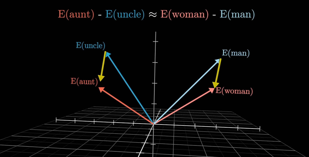
To find the female equivalent of "uncle", we can look at the vector difference between "man" and "woman", and add it to the vector for "uncle" and then see what word is nearby.
Learning encoded information on sex into one of the dimensions.

Later he gives examples. A dimension might encode "Part of a command" or "Affectionate" or "Sadness".
But normally dimensions have less clear meaning.

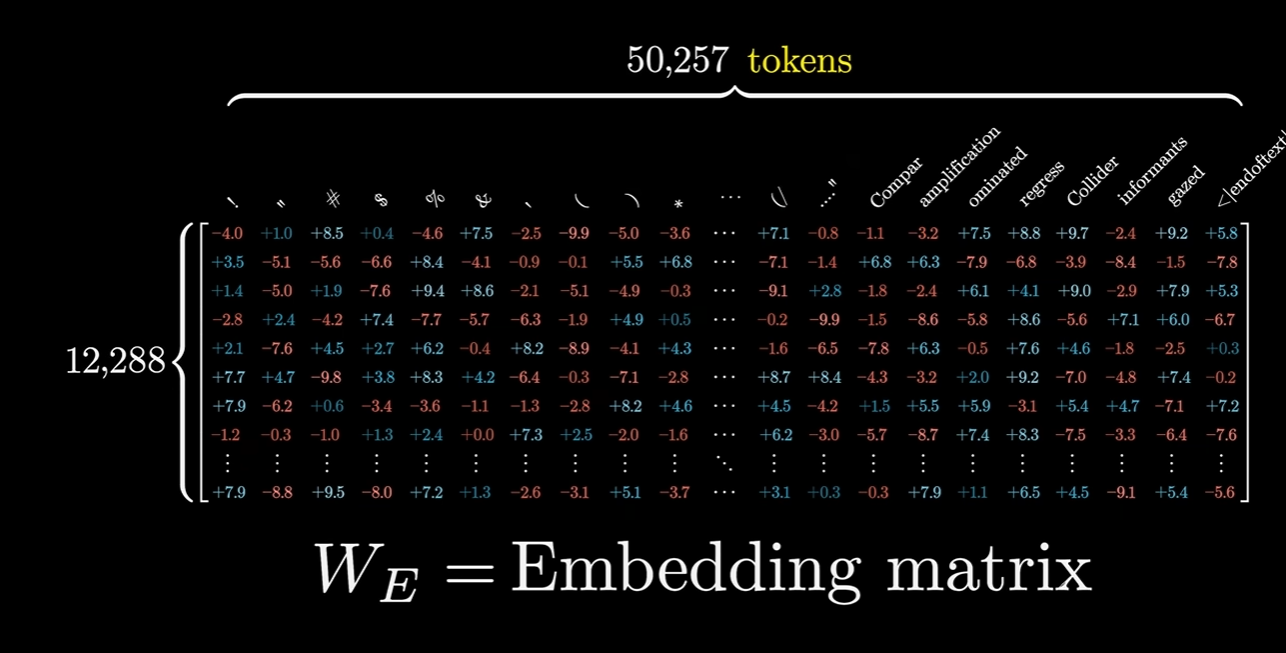
In GPT-3 there are 50,257 tokens (not exactly words) and vector length is 12,288 numbers.
That is a matrix of 617 million weights.

Vector for a word starts with its entry in the embedding matrix. Ends up being modified - for not for all instances of this word. It is for instance of word in this context.
Context size is how wide a context you can give to the tokens. How many faraway tokens can influence it.
GPT 3 context size = 2048. i.e. Data flowing through the network is 2048 columns.
The end matrix has one end column for the next token/word. The end column is combined with the unembedding matrix that maps it to a probability distribution over the tokens/words.
Unembedding matrix has a row for each token. (For GTP 3, 50,257). Columns is the same as the embedding vector size. (For GTP 3, 12,288). So again, 617 million weights.

Chapter 6: Attention in transformers

Chapter 6: Attention in transformers.

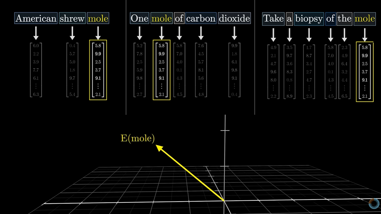
The word "mole" in 3 different sentences with 3 different meanings.
In the first step of the transformer, the word "mole" starts with the same embedding vector.
In the next step, the surrounding vectors pass information into the "mole" vector.

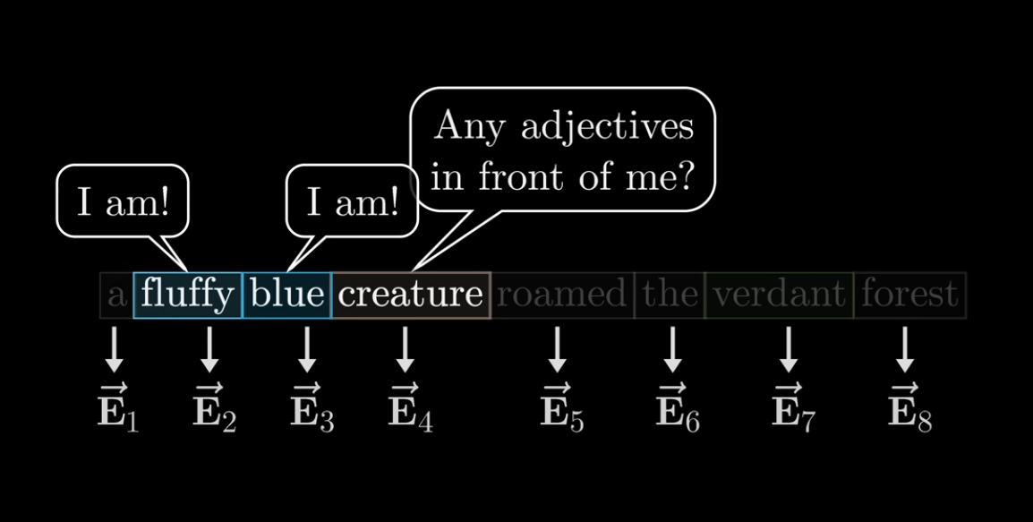
Query vector (also encoded as a vector of numbers) asks: "What information is relevant to me?"

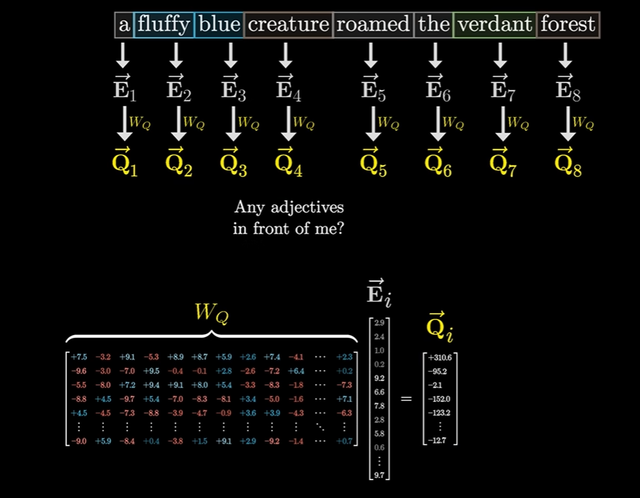
Query matrix W_Q is a matrix with learned weights to implement a query.
W_Q times (each token embedding vector) = Query vector for that token

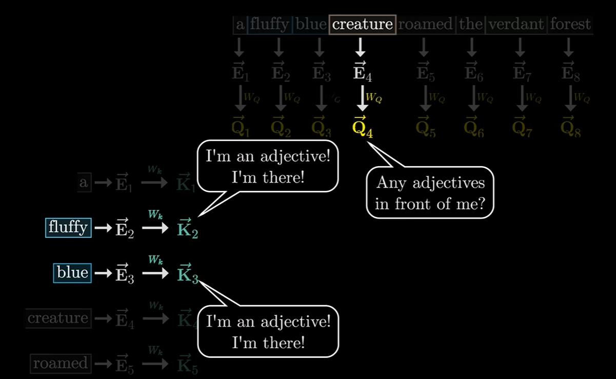
Key matrix W_K represents answers to query.
W_K times token vector = Key vector for that token

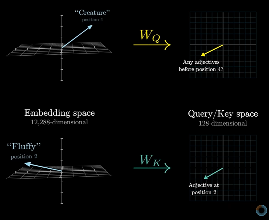
The two multiplications map the token vector into a lower dimensional space.
A match is when the key (answer) for some tokens closely matches the query (question) for the first token.

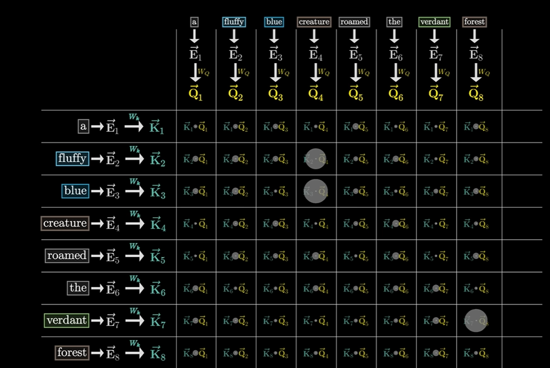
Dot product shows where queries and keys align. Result is large positive number.
The embeddings of fluffy and blue "attend to" the embedding of creature.
Softmax along column normalises values from 0 to 1. Like probability.
Get the Attention pattern for the context window.
In this version, size is square of context size.

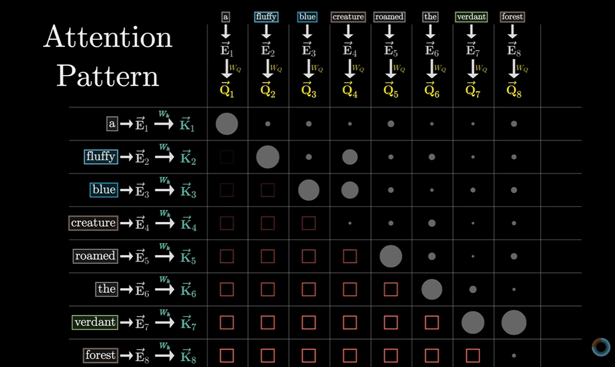
Earlier words (tokens) are meant to predict later words.
We do not want later words to influence earlier words because that breaks the prediction problem.
So we force below the diagonal here to be zero.

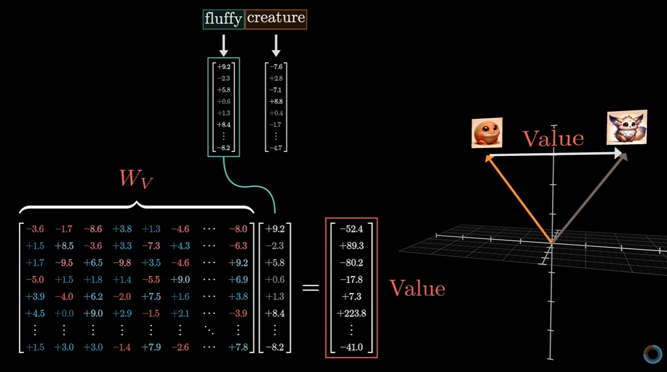
Update the embeddings.
Words relevant to other words pass information to them by adding a vector to shift their position in n-dimensional space.
Value matrix W_V times token embedding = Value vector
Value vector is added to target token embedding to move it in the space.

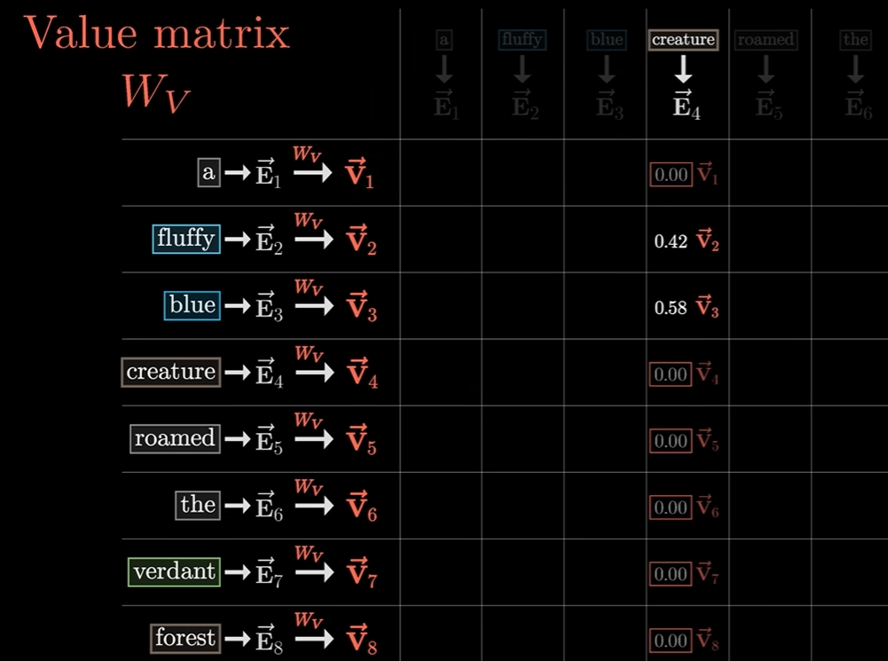
Value vector expresses: "If this token is relevant to this other token, how much should the other token be moved?"
Some tokens are part relevant, some not relevant at all.
Solution is to multiply value vector by the normalised number in the attention pattern.
Here only "blue" and "fluffy" really shift the embedding for "creature".

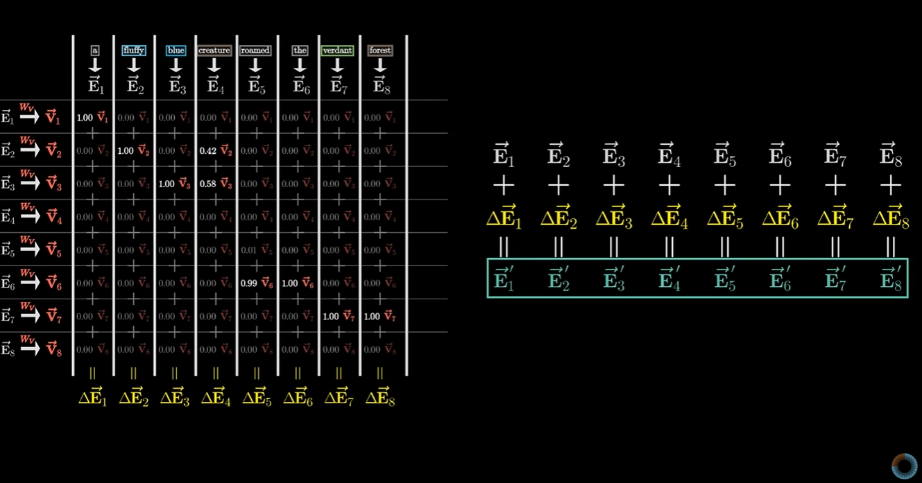
Each column shows a sum of changes (many probably near zero) to shift the vector in n-dimensional space.

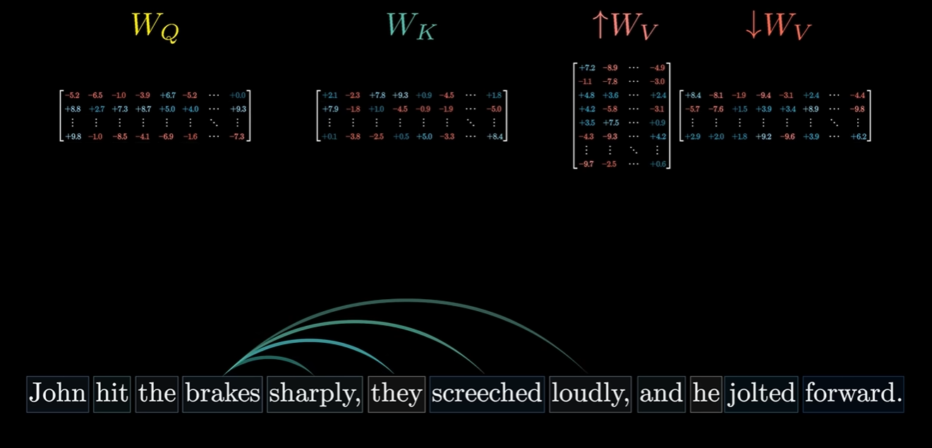
The above was for adjectives updating nouns.
For each type of contextual updating possible, we have different valued W matrices.
And what the contextual updating is is normally hard to define. The matrices are learned through training. Their function is to achieve whatever the model needs to achieve in order to predict the next token.
Multi-headed attention: Run these updates in parallel, each with its own W_Q, W_K and W_V.
GPT-3 uses 96 attention heads inside each "attention block".

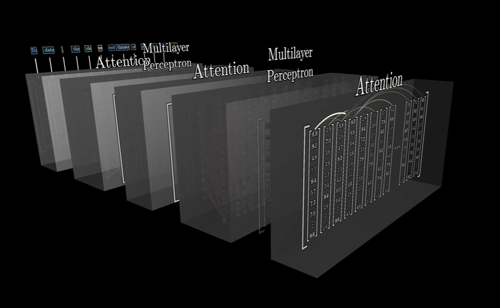
When a token vector gets updated (with extra meaning), those updates should themselves be factored in to the updates for other tokens.
So we do repeated rounds of all this. Multiple attention blocks.
Each token/word gradually takes in more meaning, in many different directions.
GPT-3 has 96 layers like this.

Chapter 7: How might LLMs store facts

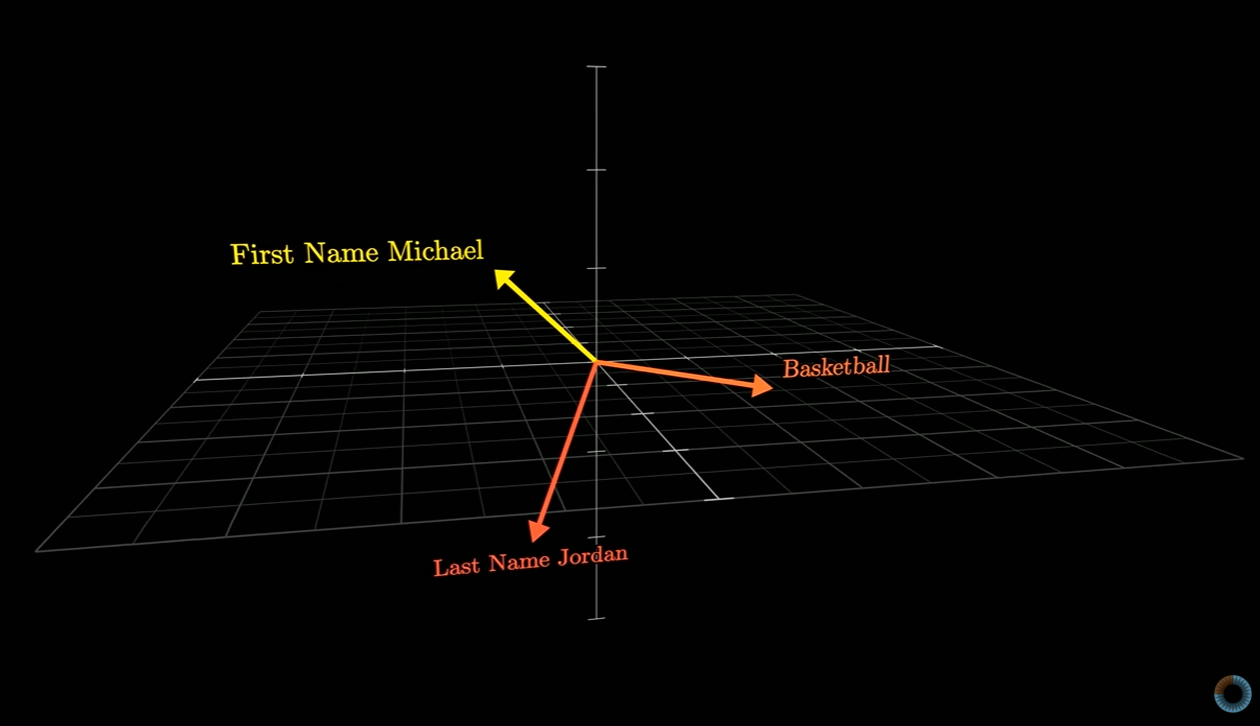
He considers how a LLM can store the fact that Michael Jordan plays basketball.
He starts by imagining that one dimension in the high dimensional space represents the idea of "First Name Michael" and another dimension represents the idea of "Last Name Jordan" and another dimension represents the idea of "basketball".
For an input string "Michael Jordan plays the sport of ...", the Attention mechanism finds "Michael" beside "Jordan", and eventually encodes into the "Jordan" vector that "Michael" is combined with it.

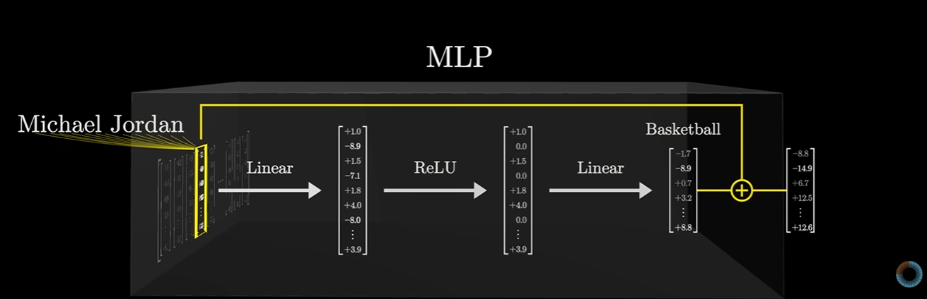
If input vector to the MLP encodes first name "Michael" and last name "Jordan" then the output of the MLP will be a vector that includes the "basketball" direction, which will be added to the original vector.

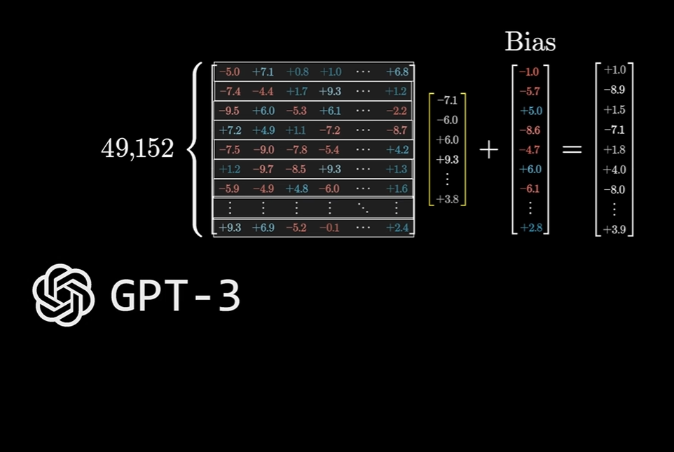
Input vector is multipled by a massive model matrix.
Each row of this essentially asks a question about the vector.
Dot product will give the answer.
In GPT-3 this has 49,152 rows.

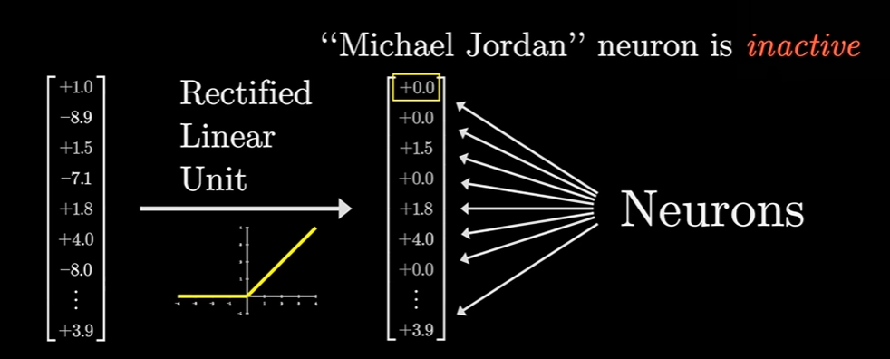
Rectifier function generates lots of zero values.
He shows where "Michael" plus "Jordan" generates 1, but one of them on their own, or neither, will generate 0.
We end up with a "Michael Jordan neuron" that is active or inactive.

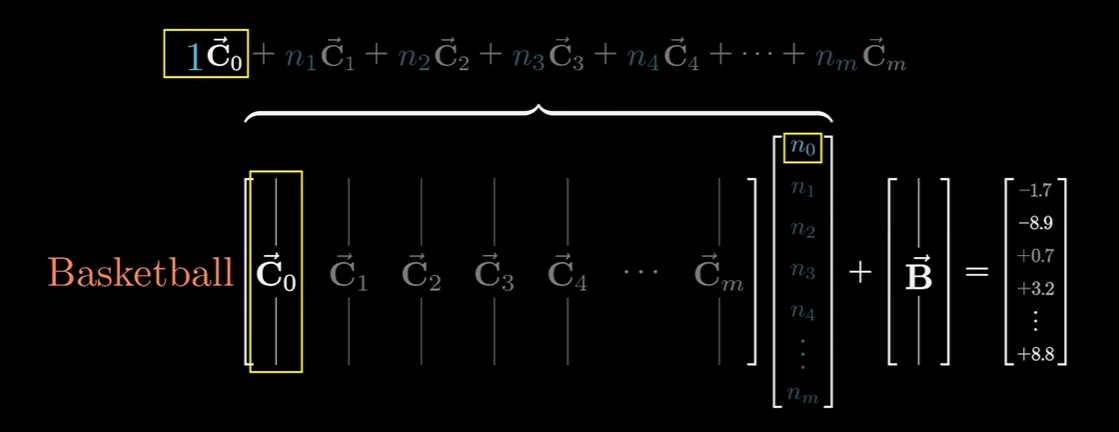
The next layer: Again multiply by a massive model matrix.
Each column can represent a set of features, like "basketball" but also other features.
If "Michael Jordan neuron" value = 1, we add this "basketball" (and other things) column to final result.
Else it = 0 and we add zero times the column to final result. i.e. No effect.

Each column shows what will be added to the final result if the corresponding neuron is active.
He then notes it is unlikely to be a single neuron for each feature.
GPT-3 has:
- 96 Attention layers. 0.6 billion parameters.
- 96 MLP layers. 1.2 billion parameters.

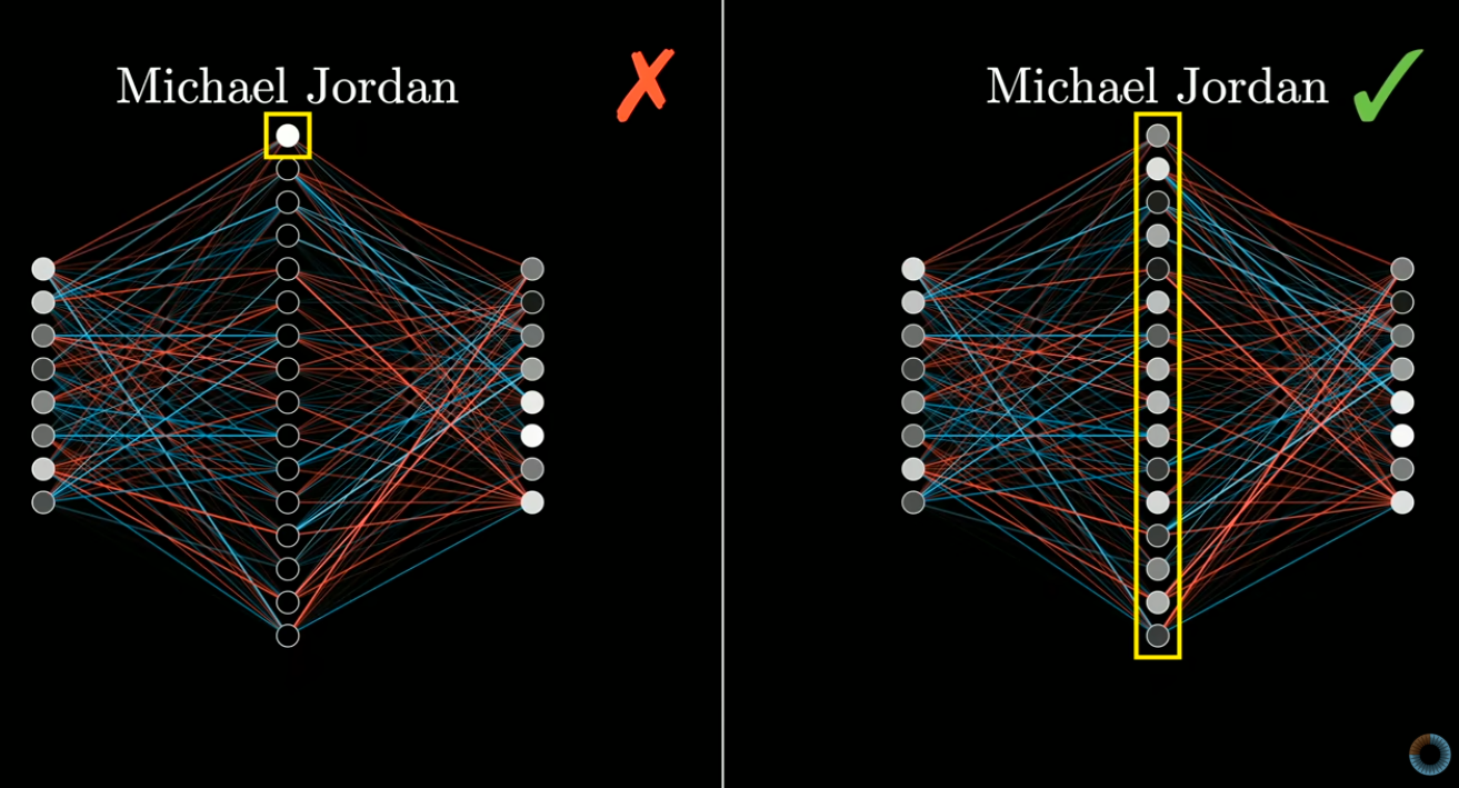
Feature recognition is unlikely to be just one neuron.